In this chapter you will learn:
- how to setup Jupyter notebook,
- how to build two ML algorithms,
- save pre-processing details and algorithms.
Setup Jupyter notebook
For building ML algorithms I’m using Jupyter notebook. It can be easily installed:
# run commands in your project directory
pip3 install jupyter notebook
To set Jupyter to use local virtualenv environment run:
ipython kernel install --user --name=venv
I will create a research directory where I will put Jupiter files. To start Jupyter notebook run:
# create a research directory
mkdir research
cd research
# start Jupyter
jupyter notebook
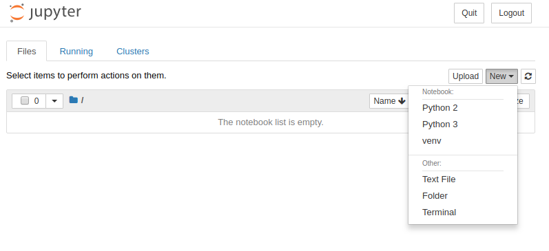
When starting a new notebook make sure that you select the correct kernel, venv in our case:
Train ML algorithms
Before building ML algorithms we need to install packages:
pip3 install numpy pandas sklearn joblib
The numpy and pandas packages are used for data manipulation. The joblib is used for ML objects saving. Whereas, the sklearn package offers a wide range of ML algorithms. We need to reload Jupyter after installation.
The first step in our code is to load packages:
import json # will be needed for saving preprocessing details
import numpy as np # for data manipulation
import pandas as pd # for data manipulation
from sklearn.model_selection import train_test_split # will be used for data split
from sklearn.preprocessing import LabelEncoder # for preprocessing
from sklearn.ensemble import RandomForestClassifier # for training the algorithm
from sklearn.ensemble import ExtraTreesClassifier # for training the algorithm
import joblib # for saving algorithm and preprocessing objects
Loading data
In this tutorial, I will use Adult Income data set. In this data set, the ML will be used to predict whether income exceeds $50K/year based on census data. I will load data from my public repository with data sets good for start with ML.
Code to load data and image with first rows of data:
# load dataset
df = pd.read_csv('https://raw.githubusercontent.com/pplonski/datasets-for-start/master/adult/data.csv', skipinitialspace=True)
x_cols = [c for c in df.columns if c != 'income']
# set input matrix and target column
X = df[x_cols]
y = df['income']
# show first rows of data
df.head()
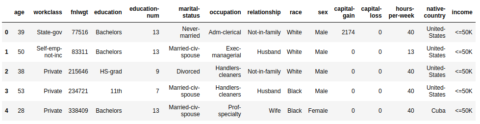
The X matrix has 32,561 rows and 14 columns. This is input data for our algorithm, each row describes one person. The y vector has 32,561 values indicating whether income exceeds 50K per year.
Before starting data preprocessing we will split our data into training, and testing subsets. We will use 30% of the data for testing.
# data split train / test
X_train, X_test, y_train, y_test = train_test_split(X, y, test_size = 0.3, random_state=1234)
Data pre-processing
In our data set, there are missing values and categorical columns. For ML algorithm training I will use the Random Forest algorithm from the sklearn package. In the current implementation it can not handle missing values and categorical columns, that’s why we need to apply pre-processing algorithms.
To fill missing values we will use the most frequent value in each column (there are many other filling methods, the one I select is just for example purposes).
# fill missing values
train_mode = dict(X_train.mode().iloc[0])
X_train = X_train.fillna(train_mode)
print(train_mode)
The train_mode values look like:
{'age': 31.0,
 'workclass': 3.0,
 'fnlwgt': 121124.0,
 'education': 11.0,
 'education-num': 9.0,
 'marital-status': 2.0,
 'occupation': 9.0,
 'relationship': 0.0,
 'race': 4.0,
 'sex': 1.0,
 'capital-gain': 0.0,
 'capital-loss': 0.0,
 'hours-per-week': 40.0,
 'native-country': 37.0}
From train_mode you see, that for example in the age column the most frequent value is 31.0.
Let’s convert categoricals into numbers. I will use LabelEncoder from sklearn package:
# convert categoricals
encoders = {}
for column in ['workclass', 'education', 'marital-status',
                'occupation', 'relationship', 'race',
                'sex','native-country']:
    categorical_convert = LabelEncoder()
    X_train[column] = categorical_convert.fit_transform(X_train[column])
    encoders[column] = categorical_convert
Algorithms training
Data is ready, so we can train our Random Forest algorithm.
# train the Random Forest algorithm
rf = RandomForestClassifier(n_estimators = 100)
rf = rf.fit(X_train, y_train)
We will also train Extra Trees algorithm:
# train the Extra Trees algorithm
et = ExtraTreesClassifier(n_estimators = 100)
et = et.fit(X_train, y_train)
As you see, training the algorithm is easy, just 2 lines of code - much less than data reading and pre-processing.
Now, let’s save the algorithm that we have created. The important thing to notice is that the ML algorithm is not only the rf and et variable (with model weights), but we also need to save pre-processing variables train_mode and encoders as well. For saving, I will use joblib package.
# save preprocessing objects and RF algorithm
joblib.dump(train_mode, "./train_mode.joblib", compress=True)
joblib.dump(encoders, "./encoders.joblib", compress=True)
joblib.dump(rf, "./random_forest.joblib", compress=True)
joblib.dump(et, "./extra_trees.joblib", compress=True)
Add ML code and artifacts to the repository
Before continuing to the next chapter, let’s add our notebook and files to the repository.
# execute in project main directory
git add research/*
git commit -am "add ML code and algorithms"
git push
Each file with preprocessing objects and algorithms is smaller than 100 MB, which is the GitHub file limit. For larger files it will be better to use separate version control systems like DVC - however, this is a more advanced topic.